- a)
MINITAB Analysis:
MATCHED PAIRS - MOTHER DAUGHTER HEIGHT EXAMPLE MTB > name c12 'dheight' (dheight is the daughter's height in inches) MTB > name c13 'mheight' (mheight is the mother's height in inches) MTB > let c20 = c12- c13 MTB > name c20 'd-m' ( d-m is the column of differences- the daughter's height minus her mother's height.) MTB > desc c12 c13 N MEAN MEDIAN TRMEAN STDEV SEMEAN dheight 30 65.000 65.000 64.962 2.807 0.512 mheight 30 64.050 63.500 63.827 2.621 0.478 MIN MAX Q1 Q3 dheight 60.000 71.000 63.000 67.000 mheight 60.000 73.000 62.000 66.000 Here are the data: ROW dheight mheight d-m 1 67.0 67.0 0.0 2 67.0 63.0 4.0 3 64.0 62.0 2.0 4 60.0 63.0 -3.0 5 71.0 68.0 3.0 6 60.0 63.0 -3.0 7 64.0 66.0 -2.0 8 68.0 64.0 4.0 9 65.0 66.0 -1.0 10 62.0 65.0 -3.0 11 68.0 65.0 3.0 12 66.0 64.0 2.0 13 70.0 73.0 -3.0 14 63.0 61.0 2.0 15 64.0 62.0 2.0 16 63.0 62.0 1.0 17 61.0 62.0 -1.0 18 66.5 62.0 4.5 19 67.0 66.0 1.0 20 64.0 64.0 0.0 21 61.0 63.0 -2.0 22 62.0 61.0 1.0 23 66.0 63.0 3.0 24 68.0 66.0 2.0 25 64.0 60.0 4.0 26 66.0 62.0 4.0 27 64.0 64.0 0.0 28 65.5 62.5 3.0 29 65.0 65.0 0.0 30 68.0 67.0 1.0 MTB > boxplot c20 (this is a boxplot of the differences d - m) If there were no difference between daughter's heights and mother's heights we would expect to see a boxplot centered on zero. That is not the case here. The median is above zero. The boxplot is fairly symmetric and there are no outliers. ---------------------------- -------------I + I---------- ---------------------------- ----+---------+---------+---------+---------+---------+--d-m -3.0 -1.5 0.0 1.5 3.0 4.5 MTB > hist c20 Histogram of d-m N = 30 Midpoint Count -3 4 **** -2 2 ** -1 2 ** 0 4 **** 1 4 **** 2 5 ***** 3 4 **** 4 4 **** 5 1 * MTB > nscores c20 c30 MTB > plot c20 c30 - * d-m - 4 - - 4 2.5+ - 5 - - 4 - 0.0+ 4 - - 2 - - 2 -2.5+ - 4 - ----+---------+---------+---------+---------+---------+--C30 -1.40 -0.70 0.00 0.70 1.40 2.10 MTB > desc c20 ( c20 is the column of differences d - m) N MEAN MEDIAN TRMEAN STDEV SEMEAN d-m 30 0.950 1.000 1.000 2.372 0.433 MIN MAX Q1 Q3 d-m -3.000 4.500 -1.000 3.000 MTB > ttest 0 c20; SUBC> alt = +1. (This specifies that we want to do a test with greater than in the alternate hypothesis.) TEST OF MU = 0.000 VS MU G.T. 0.000 N MEAN STDEV SE MEAN T P VALUE d-m 30 0.950 2.372 0.433 2.19 0.018 There is strong evidence against the null hypothesis that there is no difference on average between the heights of the mothers and their daughters. At alpha = .05 we would conclude that on average, the daughters are taller than their mothers. MTB > tint c20 N MEAN STDEV SE MEAN 95.0 PERCENT C.I. d-m 30 0.950 2.372 0.433 ( 0.064, 1.836) The 95% confidence interval tells us that the mean difference in height between daughters and their mothers is between 0.064 inches and 1.836 inches. What if we took the difference as mother's height minus daughter's height? The results are shown below. MTB > let c40 = c13-c121 MTB > name c40 'm-d' MTB > ttest 0 c40; SUBC> alt = -1. (This specifies that we want to do a test with less than in the alternate hypothesis. TEST OF MU = 0.000 VS MU L.T. 0.000 N MEAN STDEV SE MEAN T P VALUE m-d 30 -0.950 2.372 0.433 -2.19 0.018 The p-value is the same, but we had to remember to write the null hypothesis as the mean of the mother's heights is less than the mean of the daughter's heights. MTB > tint c40 N MEAN STDEV SE MEAN 95.0 PERCENT C.I. m-d 30 -0.950 2.372 0.433 ( -1.836, -0.064) The confidence interval has the same values but they are minus values because the differences are mothers height minus daughter's height, and the mothers are on average shorter. The 95% confidence interval tells us that the mean difference in height between daughters and their mothers is between 0.064 inches and 1.836 inches.di = daughter's height - mother's height
 or
or
 or
or

 or
or
 or
or

Where
 = true mean height of daughters
 = true mean height of mothers
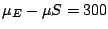
 = true mean difference in height between daughters and mothers
 ,
sd = 2.372,
nd = 30
,
sd = 2.372,
nd = 30
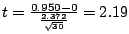
t has 29 df, 0.01 < p < 0.02
There is very strong evidence against the null hypothesis of equal height. The null hypothesis will be rejected for any
 .
.
- b)
 confidence interval for
 .
.
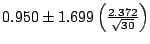
t has 29 df, t* = 1.699

(0.21 inches, 1.69 inches)
 ,
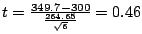
sd = 264.65, nd = 6
,
sd = 264.65, nd = 6
- a)
 or
or

 or
or

Where
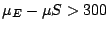
 = mean weight gain on enriched formula
 = mean weight gain on standard formula
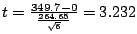 ,
t has 5 df
,
t has 5 df
0.01 < p < 0.02
At
 = 0.05 reject H0. At
= 0.01 do not reject H0.
= 0.05 reject H0. At
= 0.01 do not reject H0.
- b)
or
 or
or
t has 5 df, p > 0.25.
There is little or no evidence against the null hypothesis.
- c)
 C.I. for

t has 5 df, t* = 2.571
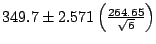

(71.92 g, 627.48 g)
The babies on enriched formula gain, on average, between 71.92 g and 627.48 g more than those on standard formula.
- d)
m = 100 g,
C.I.,
z* = 1.96,
s = 264.65 (from pilot study
of six pairs)
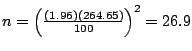 ,
need at least 27
pairs.
,
need at least 27
pairs.